1. Highway Engineer, Department of Roads, Government of Nepal, Nepal.

*             Correspondence: santapandeya@gmail.com

Keywords: Nepal, road section, F01505, F01504, India, TOPSIS, D0R

1. INTRODUCTION

For the main means of transportation for goods, people, and services are roads. And road pavement is the robust surface material set down on an area meant to withstand vehicle stress, whether a road or a walkway. As an alternative, pavement is a construction made of processed materials layered above the natural sub-grade soil. The pavement serves mostly to give the transportation economy and comfort. By the time of use, the pavement deteriorates and the degradation of these roads will first affect the transportation system with consequent negative effects on the socioeconomic activities of a nation; thus, the responsibility for proper maintenance and management of the road system by the supervising agencies. A highway agency’s main objective is to make use of public money to offer a reasonably priced, safe and comfortable road surface. To properly manage the pavements, this calls both juggling priorities and making tough decisions [1] As old as the first pavement is the idea of laying pavements and keeping them in reasonable state. Three practical phases define pavement management: inventory of all roads; regular evaluation of the conditions; and use of the condition evaluations to create project priorities [2] Pavement Management Systems (PMS) is the term used to describe correctly using these three phases in road networks. Pavement management is defined by the American Association of State Highway and Transportation Officials (AASHTO) as “the effective and efficient directing of the various activities involved in providing and sustaining pavements in a condition acceptable to the travelling public at least life cycle cost.” Designed to help decision-makers identify best strategies for preserving pavements in useable condition for a particular length of time for the least cost, a Pavement Management System is a collection of standardized procedures for gathering, assessing, managing, and reporting pavement data. Pavement failure results from the repeated motions of commercial vehicles across the surface. Considered in connection with both structural and non-structural failure influencing the comfort to the traveler is the degradation of pavement. Apart from the vehicle’s repeated movements, the pavement always degrades because of the various weather conditions [3]. The surface disturbance as well as structural collapse could result from the weather events including rainfall, sunlight, temperature variations on pavement, freeze and thaw action. Regardless of the several reasons, appropriate pavement maintenance guarantees the pavement’s structural strength and comfort for riding. The inadequate pavement maintenance system causes great vehicle operating costs (VOC) [4]. Two key treatments applied to increase pavement life as it aged are maintenance and rehabilitation. Generally speaking, maintenance helps to slow down the rate of degradation by fixing minor pavement flaws before they become more severe and support further issues. Beyond a certain point, though, flaws grow too great for repair by maintenance. By now rehabilitation can be applied for a wholesale correction of many quite serious flaws. Based on the IARMP report 2019-20 from the Department of Roads (DoR), the required budget for all kinds of maintenance projects comes out to be Nepalese Rupees 26.21 billion for national SRN. But just 6.51 billion, 25% of demand, was the authorized budget. Still a major concern is the availability of funds for SRN upkeep even after Road Board Nepal (RBN) was established in 2002 (2059) [5]. About 70% in past years (IARMP, 2019-20) the difference between demand and allocated budget is too great even after fund increase. This statistic makes it abundantly evident that budget demand and allocation vary greatly. The given money must thus be used sensibly. Dang district has 365.02 km SRN (Highway and Feeder) road overall according to DoR [6]. BT, Gravel and Earthen Road have shares of 243.02km, 100km and 22km correspondingly. Of the BT SRN road in Dang district 43% were in “Fair,” and 57% were in “Poor,” according IARMP 2019-20. This suggests that most of the roads were in “Poor,” rather than “Good,” condition. This thus calls for greater resurfacing, rehabilitation, and reconstruction efforts than for patching and crack sealing. But from the same IARMP report, rehabilitation and reconstruction receive no budgetary allocation. Routine, recurring, and periodic maintenance find their place in the budget. While regular maintenance is just for patch repairs and crack sealing, the pavement surface is not improved by the routine maintenance [7]. And part-time maintenance covers overlay projects. Two main projects to raise the state of the pavement when it reaches poor condition are rehabilitation and reconstruction. These two pieces carry the pavement on its new trip. However, for pavement in bad condition and without funding in rehabilitation and reconstruction, these road sections are more deteriorated daily as the patch repair, crack sealing and overlaying on some small sections does not provide general good quality for pavement section [8]. This suggests that next year’s demand for increased maintenance budgets will be high. The IARMP data above shows just 25% of the funds allocated in comparison to budget demand. Allocating this small budget to several road sections is absolutely vital. Still, the most important issue is which road portion will get sought budget and which route will not get it. However, all road sections should have their budget for regular maintenance and recurring maintenance divided separately; the budget for these purposes differs. Therefore, some formal method is necessary to divide this small budget in order to support the economic justification of the investment. Under such circumstances, giving road segment top priority will help to distribute the budget. Higher the priority increases the likelihood of obtaining a budget; so, budget can be distributed in line with priority [9]. It is important to take into account the several elements even while the road sections’ maintenance priorities are in development. Different elements were taken into account in the several literatures to create road maintenance’s priority. Simultaneously, all elements taken into account do not have the same weight since some may be quite significant and some less significant. Consequently, it is important to investigate the elements for prioritizing and the weightage for taken into account several elements. Under such viewpoint, this study will determine general BT SRN ranking of Dang district by considering several criteria. Budget shortage is a frequent issue in maintenance planning for Nepal. Every year, DoR implements the Annual Road Maintenance Program to gather the national SRN need for maintenance funding [11]. The RBN could not distribute the allocated funds among every road segment. This leaves the difference between allocation and budget demand. There is no way to divide this constrained budget among all the roads. DoR is thus under pressure to distribute funds on certain road without any logical basis. In this regard, road priorities are really crucial and essential. Should prioritizing be defined for every road segment, the maintenance budget can be allocated with road section priority in mind. For this reason, DoR would benefit from this kind of research in the distribution of the maintenance money [12]. Also beneficial for other road organizations for their maintenance budget planning. The development of the priorities for every BT SRN road in the Dang district is the main emphasis of this project. Only National Highway (NH) and Feeder Road Network (FRN) of the Dang area were used for the study. Using a weightage of several elements taken into account for prioritizing tool AHP, one might determine TOPSIS approach was applied to rate every BT road segment in the Dang district [13]. And this analysis also shows the scenario of limited budgets. Based on secondary data from the Highway Management and Information System- Information and Communication Technology (HMIS-ICT), DoR (2019/20 data) this analysis is conducted. This study consisted on analysis using SDI value as pavement deterioration index. Not taken into account are improvement interventions during the analysis. This study overlooked influences of other elements on prioritizing since it generated the priority order based on four factors: Surface distress index, traffic volume, Strategic relevance and maintenance cost necessary. Thus, giving priority based on elements other than above four parameters still limit this study.

2. MATERIALS AND METHODS

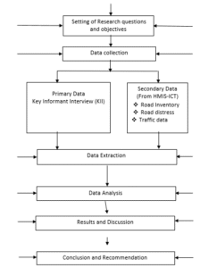
Figure 01:  Theoretical framework of study

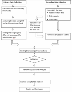
Figure 02:  Conceptual Framework of Study

First of all, from Figure 02, AHP form was developed using chosen prioritizing criteria. These AHP forms were given to KII groups. Experts from DoR, the Infrastructure Development Office of Province, and Contract Managers with road maintenance experience comprised the KII. One obtained the AHP by use of KII output analysis. TOPSIS model prioritized road sections using weightage to several elements. Following TOPSIS validation of the result form, instances including sensitivity analysis and budget deficits were established. For general success of this investigation, a quantitative method was applied. There were three phases to the research process, which have been detailed below: Pre-field work phase developed the review of literature, identification of problems, and defining of the goals of research. Major fieldwork phase tasks were gathering secondary data from several institutes and government agencies. And KII research helped to gather main data. Phase 2 Post-Fieldwork. Data analysis, conclusion and recommendation and final report preparation was done in the post field work phase.

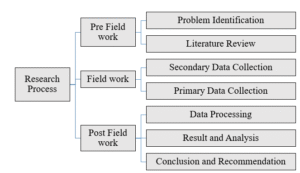
Figure 03:  Overall Research Process

The study region as depicted in Figure 04 was the Black Topped National Highways and Feeder Roads within Dang district.

Figure 04:  Study area Dang district

This study focused on road maintenance professionals in the Dang area, using all black-topped NH and FRN. The population is unknown, but 243.02 km in length. Purposive sampling was used to select key informants for the AHP. Twenty key informants were chosen for road section prioritization, including Engineer-10 from the Province Infrastructure Development Office and Superintendent Engineer-2 and Senior Divisional Engineer-8 from DoR. This study investigated road repair in Nepal using primary and secondary data from 20 professionals and sources like road inventory, traffic, and distress data. Excel documents were created, and the TOPSIS model with AHP technique was used to allocate funds in budget limitations scenarios. A consistency index and chi-square hypothesis testing validated the outcomes.

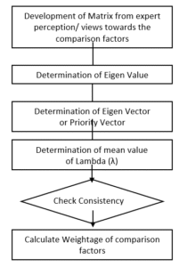
Figure 05: Flowchart for AHP Analysis

Table 01:  Pairwise Comparison Matrix obtained from Expert opinion

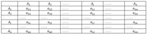
As illustrated below Aw=λw, the normalized Principal Eigen vector can be derived by averaging over the rows. λ is the average Eigenvalue of matrix A where. Now apply the formula to examine the matrix’s computed consistency. CI=(λ_max-n)/ (n-1). Where n represents matrix’s order? Given Saaty and Vargas’s (2000) reference average Random Index (RI), this Consistency Index (CI) is evaluated in Table 2.7 versus Consistency Ratio (CR) is computed by CI/ RI, the ratio of CI to the average random consistency index. The discrepancy is reasonable if the value of CR is less than 10% or equal to 10%. Should the CR be higher than 10%, the expert opinion must be changed? TOPSIS model uses this weightage as objective weight. TOPSIS Model’s determination of priority. One can obtain the choice matrix as Table 03 TOPSIS Analytical Decision Matrix A_1 x_11 x_12; B_1 B_2…… B_j……. B_n

A_2 x_21 x_22…… x_2j……. x_2n….

A_ i x_i1 x_i2……… x_ ij…… x_in ………………………………………………………………….

A_ m x_m1 x_m2…… x_ mj…… x_ mn

D equals: Where Ai = the itth alternative under consideration, Bj = the jth criterion under consideration, xij = the numerical result of the ith alternative with regard to the jth criterion. TOPSIS follows these steps: First build the normalized decision matrix by x_ ij divided by √. (∑_ (i = 1) ^ mij^2). Second step: build the weighted norma1ized decision matrix by means of w_ j×r _ ij. Third step: identify both ideal and negative-ideal solutions: Let A+ and A- be defined as two synthetic substitutes with respective meanings: [(max Vij), i=1,2, 3….m, j=1,2, 3, n] = V_ j〗^+= (V_1^+, V_2^+, V_3^+, ……V_ n^+) V_ j〗^-= (V_1^-, V_2^-, V_3^-, V_ n^-) = [(min Vij), i=1,2, 3, V_ n^-]. Fourth step: determine the separation measure. The n-dimensional Euclidean distance allows one to quantify the distances between every possibility. Then, i=1,2, 3,.m gives the separation of every alternative from the ideal one by S_ i^+= √(∑_(j=1) ^n Rye) ^2). i=1,2, 3,.m S_ i^-= √(∑_(j=1) ^n Rye (V_ ij- V_ j^-) ^2). Step 5: Determine the relative closeness to the ideal solution: C_(i+) = (S_ i^-)/ (〖 (S〗_i^++S _i^-)). Ai’s relative closeness to A+ is defined as Step 6: Sort the preference order: Ci+ allows one to rate a set of alternatives in declining order. Following TOPSIS analysis, the outcome with highest priority was validated using Kendall’s coefficient of concordance (W). First of all, utilizing AHP and TOPSIS, priority ranking of all road sections was produced for every expert’s response. The detail phases in Kendall’s coefficient of concordance (W), are First step: For every Link find the total of the ranks (R_ j) assigned by every k judge; Step 2: Find (R_j) and thereafter get s as follows: s=∑ (R_ j-(R_ j) ̅) ^ 2. Work out W’s value in step three by applying the following formula:  w= (12x s)/ (K^2 (N^3-N)) Where k= number of specialists = 20 and n= number of road links = 18? Here, n=7, Chi-Square is applied. φ=k(N-1) W Using degree of freedom equal (N – 1). The computed value of φ^2 is compared with the table value of φ^2 at 5% level for N – 1 = 18 – 1 = 17 degree of freedom; so, the appropriate selection was made. Sensitivity analysis was done to test the strength of the prioritizing after determining the final rank of every road. In Multi-attribute decision making issues, most of the data are variable instead of consistent and steady. Sensitivity analysis following problem solving can thus help to make accurate decisions rather successfully [14]. From [15], the SA process consists; Suppose ω _j, j=1, 2, 3…p…. n, is the weight to the factor “j,” then total of weights must be equal to 1. ∑_(j=1) ^nyx. Under these presumptions, the weight of one attribute changes in line with the weight of other attributes; the new vector of weights changed into ω _ j〗^’, j=1,2,3…p… n. Suppose ∆_p is the weight change to parameter p; then, new weight to parameter p is obtained by ω _p〗. ^’=ω _p +/-∆_p. New weights to remaining parameter are now obtained from ω_ j^’= (1-〖ω_ p〗^’)/〖1-ω〗_p. Sum of new altered weights has to equal 1 ∑_(j=1) ^nyx ω _j’=1〗. one these fresh weights are computed; one more new ranking is computed.

Table 02: Research Matrix

S. N	Objectives	Data required	Data Analysis
i	To determine the weightage of factors that are considered for prioritization of road sections for maintenance activities	Primary data: KII for AHP Form	AHP tool was used to determine weightage to different factors
ii	To determine priority order of road sections within Dang district using TOPSIS method	1) Secondary data: SDI, Traffic data and Importance factor 2) Maintenance cost of each road link was calculated from distress data. 3)Weightage to above factors from objective number 1	TOPSIS method was used to calculate priority order of road links
iii	To determine the most sensitive and least sensitive factor	Weightage from objective number 1 and data from objective number 2	Sensitivity analysis in Excel sheet
iv	To access how the prioritization helps to solve the problem of budget constraint	Maintenance cost of each road link and Priority ranking from objective number 2	The required maintenance budget was distributed according to priority index. For this excel as well as GIS was used to illustrate result

3. RESULT & DISCUSSION

Twenty experts from various departments, including the Department of Roads and Province Infrastructure Development Office, were given AHP forms for KII to access weightage.

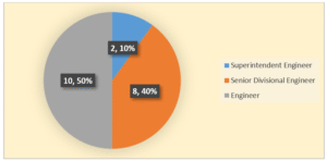
Figure 06: Composition of Key Informants

Four elements—SDI, AADT, SI and Maintenance Cost Required—were taken into consideration for road section prioritizing from the part on the literature research 2.5. For every expert, the comparison matrix tables were created based on Saaty’s Scale using their important judgment—that of pair wise comparison—against the criteria.

Table 03: Comparison Matrix for each criterion

	A	B	C	D
A	1.00	1.83	1.98	1.98
B	0.55	1.00	1.69	1.52
C	0.50	0.59	1.00	1.57
D	0.50	0.66	0.64	1.00
Sum	2.55	4.08	5.31	6.07

Were,

A= Surface distress index

B= Traffic Volume, AADT

C= Strategic Importance

D= Maintenance cost required

The geometric mean of ratings from various experts was computed, resulting in a matrix of 1.83. The AHP study showed the same values. The eigenvector was computed by dividing the summation values of each column from A to D, resulting in a matrix with eigenvalues of 0.39 and 2.55, as shown in Table 04.

Table 04:  Calculation of Eigenvector of matrix

	A	B	C	D
A	0.39	0.45	0.37	0.33
B	0.21	0.25	0.32	0.25
C	0.20	0.14	0.19	0.26
D	0.20	0.16	0.12	0.16

Next column calculates the summing of every entry in Table 04. Since we have considered four elements, the computed each sum was divided by four to obtain average value (W). Table presents the relative weightage of every criterion. Table provides factor A to D weighting. Maintenance cost necessary “D” was discovered lowest and factor SDI “A” had relative weight highest.

Table 05:  Calculation of Relative Weightage of each criterion

	A	B	C	D	Sum	W
A	0.39	0.45	0.37	0.33	1.54	0.3850
B	0.21	0.25	0.32	0.25	1.03	0.2569
C	0.20	0.14	0.19	0.26	0.79	0.1973
D	0.20	0.16	0.12	0.16	0.64	0.1608

The computation of Eigen value Lambda (λ) requires first matrix Table to be multiplied with relative weight (W) from Table 06 to get W_s. One obtained the Eigen values Lambda (λ_ i) by multiplying W_s with 1/W. We conducted the average of Eigen values Lambda (λ_ i) which produced the necessary Eigen value Lambda (λ). The required computation of Lambda λ is depicted in Table 07.

λ_ i = W_s/W now. Where, for every row l_ i = l? W_s= Weight following matrix computation

W= relative weighted matrix

Table 06:  Calculation of Eigen value Lambda (λ)

	A	B	C	D	W			λ
A	1.00	1.83	1.98	1.98	0.3850	1.57	4.0659	4.0520
B	0.55	1.00	1.69	1.52	0.2569	1.05	4.0685
C	0.50	0.59	1.00	1.57	0.1973	0.80	4.0338
D	0.50	0.66	0.64	1.00	0.1608	0.65	4.0398

Consistency Ratio (CR) =  …………. (a)

And,   …………… (b)

From Table 4.4, λ= 4.052 and m=4

 From equation (b), CI= 0.0173

Since m=4 from Table 2.6, Random Index, RI=0.9

From equation (a), CR =   =  = 0.02<0.1

Consistency ration at this is 0.02, less than 0.1. It so satisfies the consistency standards. This implies that every expert assigned their rating based on similar criteria.  The weightage to each parameter was finalised after verifying the consistency ratio test of relative weight matrix, whose value is less than 0.1. Table 07 shows the respective weight of every criterion following analysis in the AHP tool.

Table 07:  Summary of AHP Process

Criteria	Surface Distress Index (SDI) (w1)	Traffic Volume (AADT) (w2)	Strategic Importance (SI) (w3)	Maintenance cost required (w4)
Weightage, %	38.50	25.69	19.73	16.08

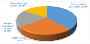
Figure 07:  Experts Weightage on Different Criteria

From the AHP study, the relative weightage to SDI was discovered as 38.50%, AADT 25.69%, SI of road 19.73% and Maintenance cost required 16.08%. Here, Maintenance cost necessary received lowest weightage and SDI received maximum weightage. This suggests that SDI has great influence in ranking of road sections and owns 38.50% equity in them. On the other hand, road section ranking is least affected by maintenance cost necessary; its participation in ranking is just 16.08%. TOPSIS model was utilized to access the Priority Index. Following sections show the detailed computation in action. Road segment priorities took SDI, AADT, SI and maintenance cost into account. Together with Table, the maintenance cost necessary was computed from the distress data [16].

Table 08: The Decision Matrix for MCDM

Link Code	SDI	AADT	SI	Maintenance Cost, NRs. in million
H0152	2.88	13601	0.60	2.47
H0154	3.00	8920	0.60	12.66
H0155	3.07	5720	0.60	239.03
H0156	2.75	2207	0.60	4.51
H0157	3.00	1913	0.60	5.21
H1101	3.07	1456	0.60	186.71
H1102	2.00	1456	0.60	14.52
H1103	2.33	5947	0.60	5.21
H1104	3.90	4114	0.60	55.29
H1726	4.00	4681	0.60	197.81
F01301	2.78	3245	0.30	18.66
F01501	2.68	3513	0.30	22.79
F01502	3.40	13007	0.30	33.75
F01503	4.00	13007	0.30	50.96
F01504	2.06	13007	0.30	0.28
F01505	4.33	13007	0.30	37.65
F14101	2.25	5608	0.30	5.58
F17901	3.83	3531	0.30	65.49

 

Table 09:  Normalized Decision Matrix

Link Code	SDI	AADT	SI	Maintenance Cost, NRs. million
H0152	0.215141	0.405006	0.288675	0.006480
H0154	0.224495	0.265617	0.288675	0.033239
H0155	0.229840	0.170328	0.288675	0.627769
H0156	0.205787	0.065719	0.288675	0.011847
H0157	0.224495	0.056965	0.288675	0.013692
H1101	0.229840	0.043356	0.288675	0.490372
H1102	0.149663	0.043356	0.288675	0.038130
H1103	0.174358	0.177088	0.288675	0.013688
H1104	0.291843	0.122505	0.288675	0.145209
H1726	0.299327	0.139389	0.288675	0.519527
F01301	0.207866	0.096629	0.144338	0.049018
F01501	0.200864	0.104609	0.144338	0.059845
F01502	0.254428	0.387319	0.144338	0.088649
F01503	0.299327	0.387319	0.144338	0.133851
F01504	0.154340	0.387319	0.144338	0.000730
F01505	0.324271	0.387319	0.144338	0.098877
F14101	0.168371	0.166993	0.144338	0.014652
F17901	0.286605	0.105145	0.144338	0.171992

Where,  = the numerical outcome of the I ^th alternative with respect to the j ^th criterion

m = Number of alternatives (number of road sections)

Table 10:  Weighted Normalized Decision Matrix

Link Code	SDI	AADT	SI	Maintenance Cost, NRs. million
H0152	0.082831	0.104062	0.056955	0.001042
H0154	0.086432	0.068247	0.056955	0.005343
H0155	0.088490	0.043764	0.056955	0.100919
H0156	0.079230	0.016886	0.056955	0.001905
H0157	0.086432	0.014636	0.056955	0.002201
H1101	0.088490	0.011140	0.056955	0.078831
H1102	0.057621	0.011140	0.056955	0.006130
H1103	0.067129	0.045501	0.056955	0.002200
H1104	0.112362	0.031476	0.056955	0.023344
H1726	0.115243	0.035814	0.056955	0.083518
F01301	0.080030	0.024828	0.028477	0.007880
F01501	0.077334	0.026878	0.028477	0.009621
F01502	0.097957	0.099517	0.028477	0.014251
F01503	0.115243	0.099517	0.028477	0.021518
F01504	0.059422	0.099517	0.028477	0.000117
F01505	0.124847	0.099517	0.028477	0.015895
F14101	0.064824	0.042907	0.028477	0.002355
F17901	0.110345	0.027016	0.028477	0.027649

 

The weighted normalized decision matrix was computed using the following equation, as presented in Table 10. v_ ij = w_ j × r_ ij w_ j represents the weightage derived from the Analytic Hierarchy Process (AHP). The weight was applied to the corresponding columns of Table 4.7 to create the weighted normalized decision matrix. Identification of Optimal and Suboptimal Solutions. The Ideal and Negative-Ideal Solutions were calculated using the following equations, and the results are presented. V_ j^+ = (V_1^+, V_2^+, V_3^+, …, V_ n^+) = [(max V_ ij), where i = 1, 2, 3, …, m and j = 1, 2, 3, …, n]  V_ j^- = (V_1^-, V_2^-, V_3^-, …, V_ n^-) = [(min V_ ij), i = 1, 2, 3, …, m, j = 1, 2, 3, …, n] .In this context, SDI, AADT, and SI are considered positive factors, while the required maintenance cost is viewed as a negative factor for prioritization. Consequently, the maximum values for SDI, AADT, and SI from Table 4.8 were designated as PIS, while the minimum values were classified as NIS. The reverse process was conducted to determine the necessary maintenance costs.

Table 11: Ideal and Negative Ideal Solutions

Solutions	SDI	AADT	SI	Maintenance Cost
Ideal (	0.1248466	0.1040617	0.0569546	0.0001173
Negative Ideal (	0.0576215	0.0111399	0.0284773	0.1009187

The separation between each alternative can be measured by following equation.

, i=1,2, 3,.m

, i=1,2, 3,.m

 

Table 12:  Separation Measure and Relative Closeness to Ideal Solution

Link Code				Ranking
H0152	0.0420	0.1416	0.7712	3
H0154	0.0528	0.1185	0.6918	5
H0155	0.1230	0.0532	0.3019	17
H0156	0.0984	0.1054	0.5172	11
H0157	0.0973	0.1068	0.5231	10
H1101	0.1271	0.0475	0.2719	18
H1102	0.1148	0.0990	0.4629	15
H1103	0.0822	0.1088	0.5694	7
H1104	0.0772	0.1012	0.5671	8
H1726	0.1082	0.0710	0.3963	16
F01301	0.0957	0.0967	0.5025	13
F01501	0.0955	0.0947	0.4980	14
F01502	0.0419	0.1302	0.7566	4
F01503	0.0372	0.1320	0.7803	2
F01504	0.0715	0.1341	0.6522	6
F01505	0.0329	0.1399	0.8097	1
F14101	0.0903	0.1038	0.5347	9
F17901	0.0878	0.0917	0.5106	12

The Coefficient of Closeness to ideal solution is given by following equation.

The final ranking of road sections is calculated from the value of C_(i+), higher the value of C_(i+) higher the priority and vice-versa. Separation Measure and Relative Closeness to Ideal Solution is given in the Table. From the TOPSIS analysis, the final ranking of road sections was obtained and is presented in Table.

Table 13:  Final Ranking of Road Sections

Ranking	Link Code	Section Name
1	F01505	Tulsipur municipality boundary-Tulsipur
2	F01503	Tribhuvannagar-Tribhuvan municipality boundary
3	H0152	Dhan Khola-Ran Singh Khola
4	F01502	Tribhuvannagar municipalityboundary-Tribhuwannagar
5	H0154	Rapti River-Bhalubang
6	F01504	Tribhuvannagar-Tulsipur municipality boundary
7	H1103	Birendrachok-Lauri Khola
8	H1104	Lauri Khola-Choroadanda, Dang district border
9	F14101	Tulasipur-Bijeneta
10	H0157	Ameliya-Shiva Khola
11	H0156	Lamahi-Ameliya
12	F17901	Ghorahi-Khumbas (Sahidmarg)
13	F01301	Bhalubang-Ganaha Khola bridge
14	F01501	Lamahi-Tribhuvannagar municipality boundary
15	H1102	Tulsipur municipality boundary-Birendrachok
16	H1726	Kalakanti (MRM)-Gadhawa-Rajpur (Postal)
17	H0155	Bhalubang-Lamahi
18	H1101	Ameliya-Tulsipur municipality boundary

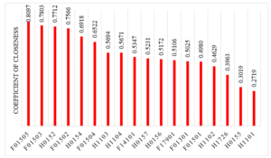
Figure 08:  Final Ranking of Road Section from TOPSIS Analysis

Table indicates that the road section Tulsipur municipality boundary-Tulsipur (F01505) exhibited the highest coefficient of closeness, thus earning the highest rank. The road section Ameliya-Tulsipur municipality boundary (H1101) exhibited the lowest coefficient of closeness, resulting in its ranking as the least favorable. According to the TOPSIS analysis, Feeder roads F01505 and F01503 were ranked first and second, respectively. This is due to these road sections exhibiting the highest traffic volume (AADT), elevated SDI values, and lower associated costs compared to others, as SDI and AADT were weighted more heavily in the ranking process. Section F01504 exhibited high traffic; however, it possessed a lower SDI value, resulting in a lower ranking compared to the first and second ranks due to this diminished SDI value. Conversely, NH road sections H0155 and H1101 ranked lowest due to an SDI of 3.07 and average traffic, coupled with higher maintenance costs, which adversely affected their ranking. Road section H1726 exhibited an SDI of 4, yet ranked third from last, primarily attributable to elevated maintenance costs. The SDI value alone is insufficient to achieve a higher ranking. The required maintenance cost was derived from distress data analysis. The total maintenance cost derived from distress value pertains solely to the repair of distress, such as pothole patching and crack sealing. Maintenance activities are essential for the preservation of road sections. However, these maintenance activities do not improve the condition of the road surface. Consequently, overlay, rehabilitation, and reconstruction are essential actions to enhance road conditions. This indicates that the maintenance cost should be determined based on SDI values and distress data. Table presents four categories of maintenance cost requirements based on SDI values. They are as follows: • Resealing only • Resealing with local patching • Rehabilitation • Reconstruction Resealing alone and Resealing with Local Patching are derived from distress data analysis. These can be classified into a single category: yearly maintenance programs. The maintenance cost requirements are categorized into three categories and are included in Appendix 6. The total maintenance cost required was determined to be 958.59 million Nepalese rupees. The share of Resealing with Local Patch was determined to be 134.56 million rupees (14.04%), while the cost of Rehabilitation (including overlay) and Reconstruction was assessed at 824.03 million rupees (85.96%). The expense associated with resealing using a local patch pertains to the remediation of distress. Consequently, it should be submitted annually to the maintenance agency to ensure the preservation of the road section.

Table 14:  Budget Available (80%) Scenario

Link Code	Rank	Budget Demand, NRs. Million	% of Demand	Budget Allocation, NRs. million
F01505	1	37.65	3.93%	37.65
F01503	2	50.96	5.32%	50.96
H0152	3	2.47	0.26%	2.47
F01502	4	33.75	3.52%	33.75
H0154	5	12.66	1.32%	12.66
F01504	6	0.28	0.03%	0.28
H1103	7	5.21	0.54%	5.21
H1104	8	55.29	5.77%	55.29
F14101	9	5.58	0.58%	5.58
H0157	10	5.21	0.54%	5.21
H0156	11	4.51	0.47%	4.51
F17901	12	65.49	6.83%	65.49
F01301	13	18.66	1.95%	18.66
F01501	14	22.79	2.38%	22.79
H1102	15	14.52	1.51%	14.52
H1726	16	197.81	20.64%	197.81
H0155	17	239.03	24.94%	232.33
H1101	18	186.71	19.48%	1.70
Total		958.59	100%	766.87

The total maintenance cost required for all road sections was determined to be NRs. 958.59 million, with 60% of this amount, or NRs. 575.15 million, being available for maintenance. The costs for resealing and local patching were allocated, and the remaining budget was distributed based on ranking. The budget allocated for the rehabilitation and reconstruction of the road section has been redirected, with the costs for resealing and local patching being reassigned to other road projects [17]. The 40% budget reduction effect was observed solely in the last two ranked road sections, H0155 and H1101. Link H0155 received NRs. 40.61 million from a total of NRs. 239.03 million. Link H1101 received only NRs. 1.70 million.

Table 15:  Budget Available (60%) Scenario

Link Code	Rank	Demand, million	% of Demand	Allocation, million
F01505	1	37.65	3.93%	37.65
F01503	2	50.96	5.32%	50.96
H0152	3	2.47	0.26%	2.47
F01502	4	33.75	3.52%	33.75
H0154	5	12.66	1.32%	12.66
F01504	6	0.28	0.03%	0.28
H1103	7	5.21	0.54%	5.21
H1104	8	55.29	5.77%	55.29
F14101	9	5.58	0.58%	5.58
H0157	10	5.21	0.54%	5.21
H0156	11	4.51	0.47%	4.51
F17901	12	65.49	6.83%	65.49
F01301	13	18.66	1.95%	18.66
F01501	14	22.79	2.38%	22.79
H1102	15	14.52	1.51%	14.52
H1726	16	197.81	20.64%	197.81
H0155	17	239.03	24.94%	40.61
H1101	18	186.71	19.48%	1.70
Total		958.59	100%	575.15

The total maintenance cost for all road sections was NRs. 958.59 million, with 40% of the cost being NRs. 383.43 million. The remaining budget was divided among the last three ranked road sections H1726, H0155, and H1101. The budget reduction effect was only seen in the last three sections, with H1726, H0155, and H1101 receiving only NRs. 44.01 million and 2.67 million respectively.

Table 16:  Budget Available (40%) Scenario

Link Code	Rank	Budget Demand, NRs. million	% of Demand	Budget Allocation, NRs. million
F01505	1	37.65	3.93%	37.65
F01503	2	50.96	5.32%	50.96
H0152	3	2.47	0.26%	2.47
F01502	4	33.75	3.52%	33.75
H0154	5	12.66	1.32%	12.66
F01504	6	0.28	0.03%	0.28
H1103	7	5.21	0.54%	5.21
H1104	8	55.29	5.77%	55.29
F14101	9	5.58	0.58%	5.58
H0157	10	5.21	0.54%	5.21
H0156	11	4.51	0.47%	4.51
F17901	12	65.49	6.83%	65.49
F01301	13	18.66	1.95%	18.66
F01501	14	22.79	2.38%	22.79
H1102	15	14.52	1.51%	14.52
H1726	16	197.81	20.64%	44.03
H0155	17	239.03	24.94%	2.67
H1101	18	186.71	19.48%	1.70
Total		958.59	100%	383.43

The total maintenance cost for all road sections was NRs. 958.59 million, with 25% of it being NRs. 239.64 million. The remaining budget was distributed based on ranking, with road sections receiving rehabilitation and reconstruction budgets. Over half of roads received only resealing and local patching costs. The 25% budget available scenario was distributed based on road section ranking, making budget distribution easier.

Table 17:  Budget Available (25%) Scenario

Link Code			Rank	Budget Demand, Million	% of Demand	Budget Allocation, Million
F01505			1	37.65	3.93%	37.65
F01503			2	50.96	5.32%	50.96
H0152			3	2.47	0.26%	2.47
F01502			4	33.75	3.52%	33.61
H0154			5	12.66	1.32%	12.66
F01504			6	0.28	0.03%	0.28
H1103			7	5.21	0.54%	5.21
H1104			8	55.29	5.77%	7.35
F14101			9	5.58	0.58%	5.58
H0157			10	5.21	0.54%	5.21
H0156			11	4.51	0.47%	4.51
F17901			12	65.49	6.83%	13.14
F01301			13	18.66	1.95%	18.66
F01501			14	22.79	2.38%	22.79
H1102			15	14.52	1.51%	14.52
H1726			16	197.81	20.64%	0.68
H0155			17	239.03	24.94%	2.67
H1101			18	186.71	19.48%	1.70
	Total			958.59	100%	239.64

The ranking was recalculated by adjusting the weight assigned to a single parameter. In a similar manner, the weightage for each parameter was adjusted individually, and rankings were computed using the following equations. Let ω_ j, where j=1, 2, 3, n, represent the weight assigned to factor j. The sum of these weights must equal 1. Thus, we have the equation: ∑_(j=1) ^n ω_ j = 1.

Let ∆_p represent the change in weightage assigned to parameter p; thus, the updated weightage for parameter p can be expressed as ω_ p’ = ω_ p ± Δ_ p  The new weights assigned to the remaining parameters are as follows: ω_ j^’ = (1 – ω_ p^’) / (1 – ω_ p) ω_ j. The sensitivity analysis was conducted by systematically varying one parameter at a time while keeping the weight constant. The altered weight ranges from -10% to +10%. All parameter weights were adjusted, and new rankings were computed. The TOPSIS model was executed for each variation in the weights of the parameters to determine the ranking. The SA was evaluated based on the change in the final ranking of road sections [18].

Table 18:  Sensitivity Analysis based on variation

	Weights
	Surface distress index (SDI) ( ’)	Traffic Volume ( ’)	Strategic Importance of road ( ’)	Maintenance cost required ( ’)
-10	0.3465	0.2730	0.2096	0.1708
-5	0.3658	0.2650	0.2035	0.1658
-4	0.3696	0.2634	0.2022	0.1648
-3	0.3735	0.2618	0.2010	0.1638
-2	0.3773	0.2602	0.1998	0.1628
-1	0.3812	0.2585	0.1985	0.1618
0	0.3850	0.2569	0.1973	0.1608
1	0.3889	0.2553	0.1961	0.1598
2	0.3927	0.2537	0.1948	0.1587
3	0.3966	0.2521	0.1936	0.1577
4	0.4004	0.2505	0.1924	0.1567
5	0.4043	0.2489	0.1911	0.1557
10	0.4235	0.2409	0.1849	0.1507

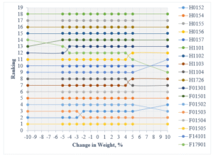
Figure 09:  Sensitivity Analysis by changing weightage

Table 19: Sensitivity Analysis based on variation of w_2

	Weights
	Surface distress index (SDI) ( ’)	Traffic Volume ( ’)	Strategic Importance of road ( ’)	Maintenance cost required ( ’)
-10	0.3983	0.2312	0.2041	0.1663
-5	0.3917	0.2441	0.2007	0.1635
-4	0.3903	0.2467	0.2000	0.1630
-3	0.3890	0.2492	0.1993	0.1624
-2	0.3877	0.2518	0.1987	0.1619
-1	0.3863	0.2544	0.1980	0.1613
0	0.3850	0.2569	0.1973	0.1608
1	0.3837	0.2595	0.1966	0.1602
2	0.3823	0.2621	0.1959	0.1596
3	0.3810	0.2646	0.1952	0.1591
4	0.3797	0.2672	0.1946	0.1585
5	0.3784	0.2698	0.1939	0.1580
10	0.3717	0.2826	0.1905	0.1552

 

 

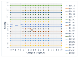
Figure 10:  Sensitivity Analysis by changing weightage 

Table 20:  Sensitivity Analysis based on variation of

	Weights
	Surface distress index (SDI) ( ’)	Traffic Volume ( ’)	Strategic Importance of road ( ’)	Maintenance cost required ( ’)
-10	0.3945	0.2633	0.1776	0.1647
-5	0.3897	0.2601	0.1874	0.1627
-4	0.3888	0.2595	0.1894	0.1623
-3	0.3878	0.2588	0.1914	0.1619
-2	0.3869	0.2582	0.1934	0.1615
-1	0.3860	0.2576	0.1953	0.1612
0	0.3850	0.2569	0.1973	0.1608
1	0.3841	0.2563	0.1993	0.1604
2	0.3831	0.2557	0.2012	0.1600
3	0.3822	0.2550	0.2032	0.1596
4	0.3812	0.2544	0.2052	0.1592
5	0.3803	0.2538	0.2072	0.1588
10	0.3755	0.2506	0.2170	0.1568

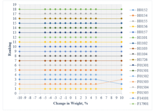
Figure 11:  Sensitivity Analysis by changing weightage

Table 21: Sensitivity Analysis based on variation of

	Weights
	Surface distress index (SDI) ( ’)	Traffic Volume ( ’)	Strategic Importance of road ( ’)	Maintenance cost required ( ’)
-10	0.3924	0.2619	0.2011	0.1447
-5	0.3887	0.2594	0.1992	0.1527
-4	0.3880	0.2589	0.1988	0.1543
-3	0.3872	0.2584	0.1984	0.1559
-2	0.3865	0.2579	0.1981	0.1575
-1	0.3857	0.2574	0.1977	0.1592
0	0.3850	0.2569	0.1973	0.1608
1	0.3843	0.2564	0.1969	0.1624
2	0.3835	0.2560	0.1965	0.1640
3	0.3828	0.2555	0.1962	0.1656
4	0.3821	0.2550	0.1958	0.1672
5	0.3813	0.2545	0.1954	0.1688
10	0.3776	0.2520	0.1935	0.1768

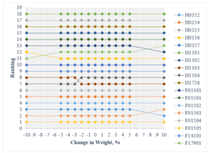
Figure 12:  Sensitivity Analysis by changing weightage

Table 22: Priority Ranking by Different Experts

Experts (E)	Ranking by different expert
	H0152	H0154	H0155	H0156	H0157	H1101	H1102	H1103	H1104	H1726	F01301	F01501	F01502	F01503	F01504	F01505	F14101	F17901
E1	1	3	18	7	8	16	12	4	14	17	10	11	6	13	2	9	5	15
E2	1	6	9	12	14	18	17	7	11	10	16	13	4	3	5	2	8	15
E3	1	6	13	10	11	18	12	7	9	15	16	14	4	3	5	2	8	17
E4	1	2	8	11	9	13	12	5	3	4	17	18	10	7	14	6	16	15
E5	1	3	18	9	10	16	13	6	14	17	11	12	4	8	2	5	7	15
E6	4	8	11	13	10	17	18	14	5	6	12	15	3	2	9	1	16	7
E7	1	6	17	10	12	18	14	7	13	16	11	9	3	5	4	2	8	15
E8	1	2	18	5	4	16	6	3	7	17	12	13	11	14	8	10	9	15
E9	5	6	18	9	8	17	15	10	3	16	11	12	4	2	13	1	14	7
E10	7	8	9	12	10	11	18	16	4	3	13	15	6	2	14	1	17	5
E11	1	6	9	15	16	18	17	7	11	10	14	13	4	3	5	2	8	12
E12	7	6	18	9	8	17	16	11	2	13	10	12	5	3	15	1	14	4
E13	4	6	17	14	11	18	15	7	9	16	12	13	3	2	5	1	8	10
E14	1	2	18	5	3	16	6	4	7	17	12	13	11	14	8	9	10	15
E15	1	2	18	5	3	16	6	4	7	17	12	13	11	14	8	9	10	15
E16	1	6	17	10	11	18	15	7	9	16	13	12	4	3	5	2	8	14
E17	1	3	18	9	8	17	14	7	11	16	12	13	4	5	6	2	10	15
E18	5	8	11	13	10	17	18	14	4	7	12	15	3	2	9	1	16	6
E19	4	6	12	16	15	18	17	7	9	10	14	13	3	2	5	1	8	11
E20	4	6	12	14	13	18	17	7	8	10	15	16	3	2	5	1	9	11

Kendall’s coefficient of concordance (W)

Step 1: For each Link determine the sum of ranks ( ) assigned by all the k judges;

Step 2: Determine  and then obtain the value of s as under:

Here,

Step 3: Work out the value of W using the following formula [19]:

Where, n= number of road link = 18, and

k= number of experts =20

.: w = 0.5904

Table 23:  Calculation of Kendall’s coefficient of concordance (W)

Link Code	Sum of Ranks,
H0152	52	19044
H0154	101	7921
H0155	289	9801
H0156	208	324
H0157	194	16
H1101	333	20449
H1102	278	7744
H1103	154	1296
H1104	160	900
H1726	253	3969
F01301	255	4225
F01501	265	5625
F01502	106	7056
F01503	109	6561
F01504	147	1849
F01505	68	14884
F14101	209	361
F17901	239	2401
		114426

4. CONCLUSION

This study focused on prioritizing road maintenance activities by evaluating four key factors: Surface Distress Index (SDI), Average Annual Daily Traffic (AADT), Strategic Importance (SI), and Maintenance Cost Required. The Analytic Hierarchy Process (AHP) was employed to assign weights to these factors through pairwise comparisons involving 20 experts. Results indicated SDI had the highest priority with a weight of 38.50%, while maintenance cost had the least priority at 16.08%. Traffic and Strategic Importance were assigned weights of 25.69% and 19.73%, respectively. The AHP analysis yielded a consistency ratio of 0.02, confirming the validity of the computation. In a subsequent TOPSIS analysis, the Tulsipur municipality boundary-Tulsipur (F01505) was ranked highest among the assessed road sections, whereas the Amelia-Tulsipur municipality (H1101) was ranked lowest. This ranking was supported by Kendall’s coefficient of concordance (W) using the χ² test, which assessed the consistency of the rankings. Maintenance costs were calculated based on distress data and SDI values, revealing a total requirement of 958.59 million Nepalese rupees for the BT SRN in Dang district. Among this, 134.56 million was allocated for resealing with local patching (14.04%), while rehabilitation and reconstruction costs made up 85.96%, totaling 824.03 million rupees. Budget scenarios were formulated for allocations of 80%, 60%, 40%, and 25%. A budget reduction of up to 40% affected the last two ranked road sections (H0155 and H1101), while a 60% budget decrease impacted the bottom three ranked sections (H1726, H0155, H1101). These three sections accounted for approximately 65% of the total maintenance budget demand. With only 25% of the budget, over half of the road sections received funding strictly for maintenance. Sensitivity analysis revealed that minor adjustments in the weight of factors SDF, AADT, SI, and maintenance costs did not significantly affect the overall ranking of the road sections. Specifically, errors in weighing factors indicated that SDI was the most sensitive parameter, while SI was the least sensitive. Recommendations from this research include prioritizing maintenance work based on weighted assessments, suggesting the Department of Roads allocate budgets according to these rankings in times of deficits, and advocating that all road maintenance considerations extend to bridges.

 REFERENCES

1. Bui, D. H. (2023). Time-Series Land Cover and Land Use Monitoring and Classification Using GIS and Remote Sensing Technology: A Case Study of Binh Duong Province, Vietnam (Doctoral dissertation, Szegedi Tudomanyegyetem (Hungary)).
2. Le Hoang, T. H., & Ly, H. T. (2024). INTEGRATING ROAD TRAFFIC SAFETY POLICY IN VIETNAM.
3. Pan, X., Dang, Y., Wang, H., Hong, D., Li, Y., & Deng, H. (2022). Resilience model and recovery strategy of transportation network based on travel OD-grid analysis. Reliability Engineering & System Safety, 223, 108483.
4. Hasibur Rashid, Md. Al Amin, Md. Tanvir Islam Khan, Nakib Rayhan, Md.Ridwanul Islam & Shahriar Azeeb (2024). Relative Comparison of Fire Resisting Capacity between Stone Aggregate Concrete and Brick Aggregate Concrete. Dinkum Journal of Natural & Scientific Innovations, 3(02):267-282.
5. Wang, C. N., Dang, T. T., & Wang, J. W. (2022). A combined Data Envelopment Analysis (DEA) and Grey Based Multiple Criteria Decision Making (G-MCDM) for solar PV power plants site selection: A case study in Vietnam. Energy Reports, 8, 1124-1142. Wang, C. N., Dang, T. T., &
6. Wang, J. W. (2022). A combined Data Envelopment Analysis (DEA) and Grey Based Multiple Criteria Decision Making (G-MCDM) for solar PV power plants site selection: A case study in Vietnam. Energy Reports, 8, 1124-1142.
7. Vieira, J., Poças Martins, J., Marques de Almeida, N., Patrício, H., & Gomes Morgado, J. (2022). Towards resilient and sustainable rail and road networks: A systematic literature review on digital twins. Sustainability, 14(12), 7060.
8. Delgado, L. R., Gomez, M., Hinojos, S., Dennis, L., & Grady, C. (2023). Investigating Social Vulnerability, Exposure, and Transport Network Disruption in the Mid-Atlantic Region. Journal of Infrastructure Systems, 29(4), 04023026.
9. Dang, H., Li, J., Zhang, Y., & Zhou, Z. (2021). Evaluation of the equity and regional management of some urban green space ecosystem services: A case study of main urban area of Xi’an City. Forests, 12(7), 813. Dang, H., Li, J., Zhang, Y., & Zhou, Z. (2021). Evaluation of the equity and regional management of some urban green space ecosystem services: A case study of main urban area of Xi’an City. Forests, 12(7), 813.
10. Krecl, P., Oukawa, G. Y., Charres, I., Targino, A. C., Grauer, A. F., & e Silva, D. C. (2022). Compilation of a city-scale black carbon emission inventory: Challenges in developing countries based on a case study in Brazil. Science of the Total Environment, 839, 156332.
11. Poudela, D. P., Shresthaa, A., Manandhara, R., Banjadea, M. R., Timsinaa, N. P., & Singhb, S. (2024). Policies for tomorrow’s risk-resilient and equitable cities. Tomorrow’s Cities (TC) & Southasia Institute of Advanced Studies (SIAS).
12. Bikash Shrestha, Dr. Bal Bahadur Parajuli, Mrs. Kumari Jyoti Joshi & Er. Aarati Thapa Magar (2024). Analysis of Variation in Compressive Strength of Hydraulic Cement Due to Curing Temperature Variations. Dinkum Journal of Natural & Scientific Innovations, 3(01):23-37.
13. Wu, G., Chen, Z., & Dang, J. (2024). Decision-Making Technologies for Intelligent Maintenance and Management. In Intelligent Bridge Maintenance and Management: Emerging Digital Technologies (pp. 403-453). Singapore: Springer Nature Singapore.
14. Faisal (2023). Water Washing System to Reduce Exhaust Odor of DI Diesel Engines at Idling. Dinkum Journal of Natural & Scientific Innovations, 2(12):852-869.
15. 함승우. (2023). Predicting the Impact on Speed Reduction in Adjacent Networks of a Link Using the Graph Attention Model (Doctoral dissertation, 서울대학교 대학원). 함승우. (2023). Predicting the Impact on Speed Reduction in Adjacent Networks of a Link Using the Graph Attention Model (Doctoral dissertation, 서울대학교 대학원).
16. OU, J., Zhang, J., Li, H., & Duan, B. Road Damage Prediction and Maintenance Optimization Method Based on Stacking Ensemble Learning. Available at SSRN 5033426. OU, J., Zhang, J., Li, H., & Duan, B. Road Damage Prediction and Maintenance Optimization Method Based on Stacking Ensemble Learning. Available at SSRN 5033426.
17. Tan, Y., Song, J., Yu, L., Bai, Y., Zhang, J., Chan, M. H., & van Ameijde, J. (2024). The mechanism of street markets fostering supportive communities in old urban districts: A case study of Sham Shui Po, Hong Kong. Land, 13(3), 289.
18. Kaisar, E. I., & Machado, A. A. (2021). Identification and Evaluation of Critical Urban and Rural Freight Corridors in the State of Florida.
19. Laanaoui, M. D., Lachgar, M., Mohamed, H., Hamid, H., Villar, S. G., & Ashraf, I. (2024). Enhancing Urban Traffic Management Through Real-Time Anomaly Detection and Load Balancing. Ieee Access.
20. Peng, F., Zhang, Z., & Ding, Q. (2024). Analysis of Guidance Signage Systems from a Complex Network Theory Perspective: A Case Study in Subway Stations. ISPRS International Journal of Geo-Information, 13(10).